CHAPTER 18
FUNCTIONS AND THEIR IMPLEMENTATION
As time goes on, we intend to program the computer with more and more
complex jobs. One of the most effective ideas in computer science is
a method of building complex programs, known as divide and
conquer. The given large problem can often be broken down into several
smaller problems. Each smaller problem can itself be broken into
several even smaller problems. Eventually, the problem size reduces
so as to be programmed in a straight-forward manner.
18.1
Functions
Each small problem can be packaged as a ~function or ~procedure.
We will use these two terms interchangeably. A function or procedure
is a program along with a name. Once you program the
small problems this way, you have a set of functions, named programs.
For example, suppose you had to compute the ~square ~root of the
~absolute ~value of a given number. The easiest approach is to break
the problem into two smaller problems, the computation of ~square ~root
and the separate computation of ~absolute ~value. Once one figures out
the arithmetic expressions for each of those two functions, one can
package each into a function. Here are the definitions for these two
functions:
DEFINE SQUARE_ROOT( X: REAL ) = REAL:
some expression using X
ENDDEFN
DEFINE ABSOLUTE_VALUE( X: REAL ) = REAL:
some expression using X
ENDDEFN
The DEFINE line in each tells the name of the function, and what
parameters it takes in (one REAL) and what it delivers (a REAL). Each
parameter is assigned a name, X in both examples. That name X becomes
a variable, which contains the input parameter.
Having in hand our two functions, we can compute the original problem.
Here is one way:
Y:= the given number ;
Y:= ABSOLUTE_VALUE( Y ) ;
Y:= SQUARE_ROOT( Y ) ;
We call a function by writing its name followed by its parameter(s)
enclosed in parentheses. Here, we call ABSOLUTE_VALUE first and pass
that result into SQUARE_ROOT. Y holds the answer in the end. We
could write this solution more briefly as:
Y:= SQUARE_ROOT( ABSOLUTE_VALUE( the given number ) ) ;
Like before, the value resulting from ABSOLUTE_VALUE is fed directly
into SQUARE_ROOT.
This chapter introduces ways to implement such function definitions
and subsequent calls to the functions.
18.1.1
Parameters
The line
DEFINE ABSOLUTE_VALUE( X: REAL ) = REAL:
indicates the name of the function and also what parameters it takes
in, one REAL called X, and what it delivers, a REAL. Recall that REAL
denotes numbers including fractions. The ~body of this function
follows the DEFINE line. It can use the variable X. Wherever X
appears in the body, the given REAL parameter will be substituted.
For example, the body is included in:
DEFINE ABSOLUTE_VALUE( X: REAL ) = REAL:
IF X < 0 THEN -X ELSE X FI
ENDDEFN
If someone writes:
ABSOLUTE_VALUE( -3 )
which ~calls the function, the body is executed where X is -3:
IF -3 < 0 THEN -(-3) ELSE -3 FI
This IF statement sees that indeed -3 is less than 0, and so it
delivers its THEN clause, the -(-3), which computes to 3. This 3 is
the result of our call to ABSOLUTE_VALUE.
Great flexibility is achieved by defining functions with parameters.
Each call to a function can take advantage of the function's different
behaviors when given different input value(s) for the parameter(s).
One program, although written only once, can be called many times.
A function definition buries details. All the detail in the
function's body becomes invisible from all points of view outside the
function definition. When we call ABSOLUTE_VALUE, the details inside
its definition are invisible.
The only thing in common between the insides and the outsides of a
function are its parameters, e.g., the REAL coming in and the REAL
coming out of ABSOLUTE_VALUE. This isolation between insides and
outsides reduces drastically the potential for bugs. Nobody outside
of ABSOLUTE_VALUE's definition can damage ABSOLUTE_VALUE's correctness.
The details of ABSOLUTE_VALUE and the details of SQUARE_ROOT remain
permanently separated.
(We wonder in Section 19.10 what happens if the function itself tries
to put a value into the parameter).
18.1.2
Local Variables
In programming the function body, one may need some extra variables.
For example, let's define the function POWER_OF_2 which takes in a
number and yields the smallest power of two which is at least as
large as the given number:
DEFINE POWER_OF_2( X: REAL ) = REAL:
DO Y:= 0;
WHILE 2^Y < X; DO Y:= Y+1 ; END
GIVE 2^Y
ENDDEFN
This function uses a variable Y, to hold possible exponents. It sets
Y to zero initially. While 2-to-the-Y'th power (2^Y) is less than X,
we increment Y. We expect that eventually 2^Y will be as large as X.
When that loop terminates, 2^Y is greater than or equal to X,
and we give 2^Y as the answer.
The variable Y deserves some attention. We intend that its use be
limited to this function alone. If this variable Y were used somewhere
as well, our use of the variable could surprise that other point of
view, as we do put new values into Y.
To assure that the variable Y is ours alone, we declare Y to be a
~local ~variable. We enclose our program that uses Y in the
BEGIN...END construct. Following the BEGIN, we declare Y to be a
variable as in:
VAR Y = INT ;
This makes Y a local variable. Here is the program:
BEGIN
VAR Y = INT ;
DO Y:= 0;
WHILE 2^Y < X; DO Y:= Y+1 ; END
GIVE 2^Y
END
Inside the BEGIN...END, we can use Y freely, and also be assured that
nowhere outside the BEGIN...END will Y be visible. The BEGIN...END
thus defines the ~scope of the VAR (variable) declarations. This
establishes us, the insides of the BEGIN...END, as the sole owners of
Y. The airtight privacy assured by the BEGIN...END makes it possible
to write large systems without interference among its variables.
BEGIN...ENDs almost always appear within function definitions, as the
outermost construct. Our POWER_OF_2 function needs the variable Y,
so we enclose the function body with a BEGIN...END:
DEFINE POWER_OF_2( X: REAL ) = REAL:
BEGIN
VAR Y = INT ;
DO Y:= 0;
WHILE 2^Y < X; DO Y:= Y+1 ; END
GIVE Y
END
ENDDEFN
The function body has access to the parameter X and also the local
variable Y. Because Y is a local variable, the sole entities shared
between the insides of this function and anyone who calls this function
is the input parameter and the output result, and not Y.
BOX: What are parameters?
BOX:
BOX: What are local variables?
BOX:
BOX: Thru which of these two does a function communicate
BOX: with its caller?
�
18.2
The Implementation Of Function Definitions And Calls
18.2.1
Pushes And Pops - The Stack
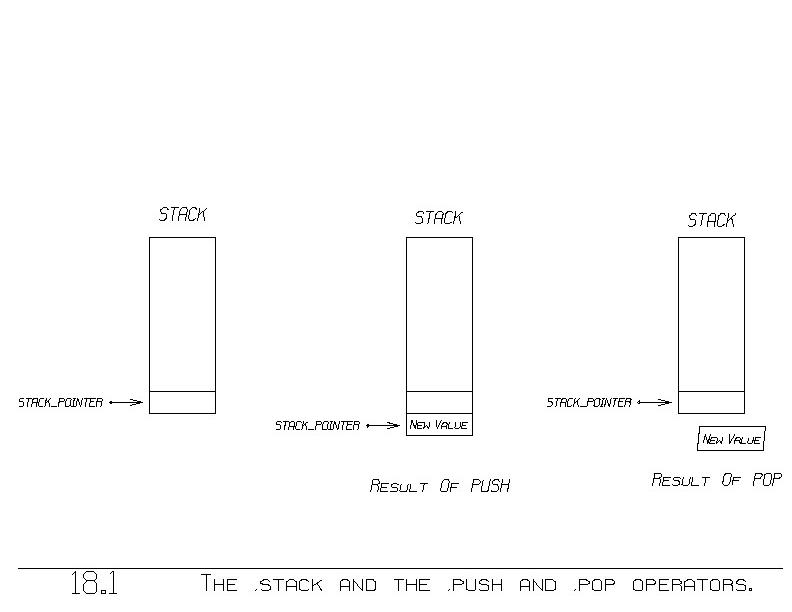 A simple and very useful method of using memory is called the ~stack.
A stack is a block of memory (figure 18.1). You can ~push a new value
onto the stack, and ~pop a value off the stack.
The push operator appends a new bin at the end of the stack (figure
18.1(b)), where it stores the new value, push's operand. For each
push, there is ultimately a corresponding pop. Pop removes the last
bin from the end of the stack and yields as its value the contents of
that last bin (figure 18.1(c)).
The last bin in the stack is referenced by what is called the ~stack
~pointer, or ~SP for short. The stack pointer always contains the
address of the bin containing the most recently pushed data. We keep
that pointer in a register called ~SP.
In assembly language, as introduced in Chapters 6 and 7 and Sections
9.5 and 9.8, the push operator is implemented as follows. We increment
the stack pointer (SP) so as to point to the next available bin. We
then store the new data into that bin:
ADD( SP , ADDRESS_OF(1) ); "Increment SP"
STORE( ~new ~value , 0 \OFF_OF SP );
"Store the given value into the
bin whose address is in SP"
The ~new ~value denotes the value that is pushed onto the stack.
(The ADD and STORE instructions were introduced in Section 6.1.4 and
the ADDRESS_OF function appears in Section 7.7.4).
The pop operator undoes the push operator. It acquires the value on
the top of the stack, to become pop's result, and then decrements SP:
LOAD( 1 , 0 \OFF_OF SP ); "Get value on stack top into
register 1"
SUB( SP , ADDRESS_OF(1) ); "Decrement SP"
The result appears in register 1 (due to the LOAD).
The pop operator fetches what's on the end of the stack, that which
was left by the most recent push operation. After the pop, the stack
is in exactly the same shape it was prior to the preceding,
corresponding push.
Our stacks push by using a bin with a ~higher (not lower) address,
(unlike the VAX). Also, many machines can perform a push or a pop as
a single instruction.
BOX: What does ~push do?
BOX:
BOX: What does ~pop do?
BOX:
BOX: Are pushes always related to corresponding pops?
BOX:
BOX: What might happen if someone forgets to ~pop a pushed
BOX: value?
18.2.2
Calling Functions
We first consider the calling of functions ignoring both parameters
and local variables. We will introduce these shortly.
Machines generally have a special instruction for calling functions,
named CALL. It takes two operands, as follows:
CALL( register , address of program we are calling ) ;
This instruction is just like a JUMP in that it jumps to the address
given as the second operand. That address is presumed to be the
beginning of the called function's machine language program.
A simple and very useful method of using memory is called the ~stack.
A stack is a block of memory (figure 18.1). You can ~push a new value
onto the stack, and ~pop a value off the stack.
The push operator appends a new bin at the end of the stack (figure
18.1(b)), where it stores the new value, push's operand. For each
push, there is ultimately a corresponding pop. Pop removes the last
bin from the end of the stack and yields as its value the contents of
that last bin (figure 18.1(c)).
The last bin in the stack is referenced by what is called the ~stack
~pointer, or ~SP for short. The stack pointer always contains the
address of the bin containing the most recently pushed data. We keep
that pointer in a register called ~SP.
In assembly language, as introduced in Chapters 6 and 7 and Sections
9.5 and 9.8, the push operator is implemented as follows. We increment
the stack pointer (SP) so as to point to the next available bin. We
then store the new data into that bin:
ADD( SP , ADDRESS_OF(1) ); "Increment SP"
STORE( ~new ~value , 0 \OFF_OF SP );
"Store the given value into the
bin whose address is in SP"
The ~new ~value denotes the value that is pushed onto the stack.
(The ADD and STORE instructions were introduced in Section 6.1.4 and
the ADDRESS_OF function appears in Section 7.7.4).
The pop operator undoes the push operator. It acquires the value on
the top of the stack, to become pop's result, and then decrements SP:
LOAD( 1 , 0 \OFF_OF SP ); "Get value on stack top into
register 1"
SUB( SP , ADDRESS_OF(1) ); "Decrement SP"
The result appears in register 1 (due to the LOAD).
The pop operator fetches what's on the end of the stack, that which
was left by the most recent push operation. After the pop, the stack
is in exactly the same shape it was prior to the preceding,
corresponding push.
Our stacks push by using a bin with a ~higher (not lower) address,
(unlike the VAX). Also, many machines can perform a push or a pop as
a single instruction.
BOX: What does ~push do?
BOX:
BOX: What does ~pop do?
BOX:
BOX: Are pushes always related to corresponding pops?
BOX:
BOX: What might happen if someone forgets to ~pop a pushed
BOX: value?
18.2.2
Calling Functions
We first consider the calling of functions ignoring both parameters
and local variables. We will introduce these shortly.
Machines generally have a special instruction for calling functions,
named CALL. It takes two operands, as follows:
CALL( register , address of program we are calling ) ;
This instruction is just like a JUMP in that it jumps to the address
given as the second operand. That address is presumed to be the
beginning of the called function's machine language program.
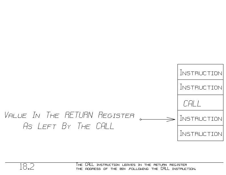 Besides jumping, the CALL instruction puts the ~return ~address into
the register. We call that register the ~return register. The return
address is always the address of the bin following the bin containing
the CALL instruction (figure 18.2).
The called function, when it is done, will JUMP back to the address
contained in that register. This will cause program execution to
resume at the bin following the CALL instruction. That is precisely
where we want program execution to resume after the called function is
finished.
Let's agree to use always the same register in all CALL instructions.
Let RETURN denote that one register. We call a function by executing:
CALL( RETURN , address of program );
To respond to the CALL, we will introduce at the end of each function
body an extra instruction to cause the function to return:
JUMP( 0 \OFF_OF RETURN );
This JUMP instruction jumps to the address in RETURN, which was set up
by the CALL instructions. (The address expression "0 \OFF_OF RETURN"
denotes the return address, the address in RETURN). Thus, the last
thing a function does is to jump back to the instruction following
the CALL instruction that got this function started.
18.2.2.1
Saving RETURN
We would be all done if it weren't for the fact that one function may
call another function. Consider the following function definition:
DEFINE FUNCTION1:
...
FUNCTION2;
...
ENDDEFN
FUNCTION1 calls FUNCTION2.
In assembly language, FUNCTION1 appears as:
FUNCTION1: ...
CALL( RETURN , FUNCTION2 ); "the call to FUNCTION2"
... "Oops!"
...
JUMP( 0 \OFF_OF RETURN ); "the return from FUNCTION1"
Recall that upon entry to FUNCTION1, RETURN points to where FUNCTION1
should return. Unfortunately, FUNCTION1's call to FUNCTION2 damages
the contents of register RETURN. After executing this CALL, and after
FUNCTION2 returns, RETURN will naturally contain the address of the
bin following this CALL instruction. That ~isn't the address where we,
FUNCTION1, are supposed to return.
In fact, upon executing our JUMP to return, we will not go back to from
where FUNCTION1 was called, but instead we will go back to the bin
following the most recently executed CALL instruction. That most
recently executed CALL instruction is our call to FUNCTION2. Thus,
upon executing our final JUMP instruction, we will go to the point in
our program labelled "Oops!". We will never return. We will
reexecute the tail of this program forever!
Clearly, if we call another function, we must protect the present
contents of the register RETURN. Immediately upon entry to a function,
we will push RETURN onto the stack. Also, just prior to the return
JUMP instruction, we will pop RETURN off the stack. Because we save
and then restore RETURN, in the interim RETURN can be used for other
purposes, such as calling other functions.
We now write FUNCTION1 as:
FUNCTION1: "push RETURN onto the top of the stack:"
ADD( SP , ADDRESS_OF(1) );
STORE( RETURN, 0 \OFF_OF SP );
"The function body:"
...
CALL( RETURN, FUNCTION2 ); "(a call to another
function)"
...
"Our correct return:"
"Pop the stack so as to restore our return address
into RETURN:"
LOAD( RETURN , 0 \OFF_OF SP );
SUB( SP , ADDRESS_OF(1) );
" Return now: "
JUMP( 0 \OFF_OF RETURN );
We save our RETURN address on the stack, and then restore it at the
end, when we need to return. This saving and restoring allows us to
make calls to other functions, and still remember our particular
return address.
FUNCTION1 can even call itself safely. For example, substitute the
appearence of FUNCTION2 by FUNCTION1. When we call ourself, this
second incarnation of ourself saves its return address on the stack,
at a ~higher ~bin than the one used by our first incarnation. A
higher bin is used because we incremented SP each time we enter the
function. Thus all of our incarnations each saves its return address
in a different bin, and hence all return correctly to where each had
been called from.
We now establish the convention that upon return from a called
function, ~the ~stack ~appears ~unchanged. We've made this so by
popping the stack upon return, to undo the push at the beginning.
This stack invariant is in fact necessary. We expect SP to ~remain
~unchanged upon each function call, because we restore RETURN from an
address expression involving SP.
BOX: Why must RETURN be saved?
BOX:
BOX: Why can one function call itself recursively and
BOX: still be able to return correctly in each instance?
18.2.3
Passing Parameters
We pass a parameter to a function by pushing the value onto the stack
~prior to calling the function.
For example, we call POWER_OF_2, which takes one parameter, by:
"Push the parameter onto the stack:"
ADD( SP , ADDRESS_OF(1) );
STORE( parameter_value , 0 \OFF_OF SP );
"The call:"
CALL( RETURN , POWER_OF_2 );
The first thing that POWER_OF_2 does, of course, is to save RETURN on
the stack:
POWER_OF_2: ADD( SP, ADDRESS_OF(1) );
STORE( RETURN , 0 \OFF_OF SP );
"the body:"
...
Besides jumping, the CALL instruction puts the ~return ~address into
the register. We call that register the ~return register. The return
address is always the address of the bin following the bin containing
the CALL instruction (figure 18.2).
The called function, when it is done, will JUMP back to the address
contained in that register. This will cause program execution to
resume at the bin following the CALL instruction. That is precisely
where we want program execution to resume after the called function is
finished.
Let's agree to use always the same register in all CALL instructions.
Let RETURN denote that one register. We call a function by executing:
CALL( RETURN , address of program );
To respond to the CALL, we will introduce at the end of each function
body an extra instruction to cause the function to return:
JUMP( 0 \OFF_OF RETURN );
This JUMP instruction jumps to the address in RETURN, which was set up
by the CALL instructions. (The address expression "0 \OFF_OF RETURN"
denotes the return address, the address in RETURN). Thus, the last
thing a function does is to jump back to the instruction following
the CALL instruction that got this function started.
18.2.2.1
Saving RETURN
We would be all done if it weren't for the fact that one function may
call another function. Consider the following function definition:
DEFINE FUNCTION1:
...
FUNCTION2;
...
ENDDEFN
FUNCTION1 calls FUNCTION2.
In assembly language, FUNCTION1 appears as:
FUNCTION1: ...
CALL( RETURN , FUNCTION2 ); "the call to FUNCTION2"
... "Oops!"
...
JUMP( 0 \OFF_OF RETURN ); "the return from FUNCTION1"
Recall that upon entry to FUNCTION1, RETURN points to where FUNCTION1
should return. Unfortunately, FUNCTION1's call to FUNCTION2 damages
the contents of register RETURN. After executing this CALL, and after
FUNCTION2 returns, RETURN will naturally contain the address of the
bin following this CALL instruction. That ~isn't the address where we,
FUNCTION1, are supposed to return.
In fact, upon executing our JUMP to return, we will not go back to from
where FUNCTION1 was called, but instead we will go back to the bin
following the most recently executed CALL instruction. That most
recently executed CALL instruction is our call to FUNCTION2. Thus,
upon executing our final JUMP instruction, we will go to the point in
our program labelled "Oops!". We will never return. We will
reexecute the tail of this program forever!
Clearly, if we call another function, we must protect the present
contents of the register RETURN. Immediately upon entry to a function,
we will push RETURN onto the stack. Also, just prior to the return
JUMP instruction, we will pop RETURN off the stack. Because we save
and then restore RETURN, in the interim RETURN can be used for other
purposes, such as calling other functions.
We now write FUNCTION1 as:
FUNCTION1: "push RETURN onto the top of the stack:"
ADD( SP , ADDRESS_OF(1) );
STORE( RETURN, 0 \OFF_OF SP );
"The function body:"
...
CALL( RETURN, FUNCTION2 ); "(a call to another
function)"
...
"Our correct return:"
"Pop the stack so as to restore our return address
into RETURN:"
LOAD( RETURN , 0 \OFF_OF SP );
SUB( SP , ADDRESS_OF(1) );
" Return now: "
JUMP( 0 \OFF_OF RETURN );
We save our RETURN address on the stack, and then restore it at the
end, when we need to return. This saving and restoring allows us to
make calls to other functions, and still remember our particular
return address.
FUNCTION1 can even call itself safely. For example, substitute the
appearence of FUNCTION2 by FUNCTION1. When we call ourself, this
second incarnation of ourself saves its return address on the stack,
at a ~higher ~bin than the one used by our first incarnation. A
higher bin is used because we incremented SP each time we enter the
function. Thus all of our incarnations each saves its return address
in a different bin, and hence all return correctly to where each had
been called from.
We now establish the convention that upon return from a called
function, ~the ~stack ~appears ~unchanged. We've made this so by
popping the stack upon return, to undo the push at the beginning.
This stack invariant is in fact necessary. We expect SP to ~remain
~unchanged upon each function call, because we restore RETURN from an
address expression involving SP.
BOX: Why must RETURN be saved?
BOX:
BOX: Why can one function call itself recursively and
BOX: still be able to return correctly in each instance?
18.2.3
Passing Parameters
We pass a parameter to a function by pushing the value onto the stack
~prior to calling the function.
For example, we call POWER_OF_2, which takes one parameter, by:
"Push the parameter onto the stack:"
ADD( SP , ADDRESS_OF(1) );
STORE( parameter_value , 0 \OFF_OF SP );
"The call:"
CALL( RETURN , POWER_OF_2 );
The first thing that POWER_OF_2 does, of course, is to save RETURN on
the stack:
POWER_OF_2: ADD( SP, ADDRESS_OF(1) );
STORE( RETURN , 0 \OFF_OF SP );
"the body:"
...
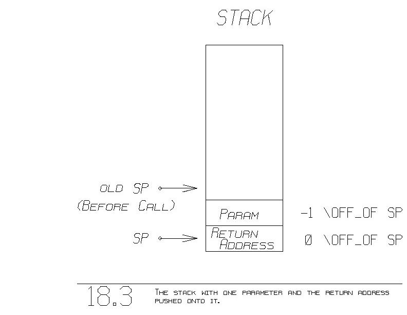 Upon finally entering "the body", the stack looks like figure 18.3. We
have pushed onto the stack both the parameter and our return address.
At this point, the parameter resides at "-1 \OFF_OF SP" and the return
address is in "0 \OFF_OF SP".
In our definition of POWER_OF_2, we specified that X will be the name
by which we will refer to the parameter. (See how X appeared on the
DEFINE line). Let's associate with X the address expression
"-1 \OFF_OF SP", so that wherever X appears in the function's body,
we substitute X with this address expression.
Thus, we translate:
Y:= X*X ;
into:
LOAD( 1, -1 \OFF_OF SP ); "Get X into register 1"
MUL( 1, -1 \OFF_OF SP ); "X*X in register 1"
STORE( 1, Y );
18.2.3.1
Returning Pops The Parameters Off The Stack
Upon return, POWER_OF_2, like any function, must restore its return
address by popping it off the stack. Not only must it pop the return
address, it must also pop the parameter off the stack. This is
necessary so as to leave the stack appearing unchanged.
Before the full call, the parameter and the return address were ~not
on the stack.
Thus, the entirety of POWER_OF_2 looks like the following. Recall
that upon entry here, the one parameter has already been pushed onto
the stack.
POWER_OF_2: "push RETURN on to the stack:"
ADD( SP , ADDRESS_OF(1) );
STORE( RETURN, 0 \OFF_OF SP );
"Now both the parameter and the return address are on
the stack."
"the body:"
...
"the return:"
LOAD( RETURN, 0 \OFF_OF SP ); "Grab RETURN off stack"
SUB( SP , ADDRESS_OF( 2 ) ); "Pop ~both the return
address and parameter
off the stack"
JUMP( 0 \OFF_OF RETURN );
Notice that we decrement SP by 2 at the end. This effectively pops
off both the return address and the parameter.
Our conventions used so far are summarized:
1) Upon calling a function:
a) Push the parameter(s) onto the stack
b) CALL the function, leaving the return address in
register RETURN.
2) Upon entry into a function:
a) Push RETURN onto the stack
3) Upon exit from the function:
a) Pop RETURN off the stack
b) Decrement SP (the stack pointer) so as to effectively
pop off all the parameters as well.
Indeed, each full call, including parameter passing, leaves the stack
appearing unchanged upon return.
18.2.4
Multiple Parameters
Upon finally entering "the body", the stack looks like figure 18.3. We
have pushed onto the stack both the parameter and our return address.
At this point, the parameter resides at "-1 \OFF_OF SP" and the return
address is in "0 \OFF_OF SP".
In our definition of POWER_OF_2, we specified that X will be the name
by which we will refer to the parameter. (See how X appeared on the
DEFINE line). Let's associate with X the address expression
"-1 \OFF_OF SP", so that wherever X appears in the function's body,
we substitute X with this address expression.
Thus, we translate:
Y:= X*X ;
into:
LOAD( 1, -1 \OFF_OF SP ); "Get X into register 1"
MUL( 1, -1 \OFF_OF SP ); "X*X in register 1"
STORE( 1, Y );
18.2.3.1
Returning Pops The Parameters Off The Stack
Upon return, POWER_OF_2, like any function, must restore its return
address by popping it off the stack. Not only must it pop the return
address, it must also pop the parameter off the stack. This is
necessary so as to leave the stack appearing unchanged.
Before the full call, the parameter and the return address were ~not
on the stack.
Thus, the entirety of POWER_OF_2 looks like the following. Recall
that upon entry here, the one parameter has already been pushed onto
the stack.
POWER_OF_2: "push RETURN on to the stack:"
ADD( SP , ADDRESS_OF(1) );
STORE( RETURN, 0 \OFF_OF SP );
"Now both the parameter and the return address are on
the stack."
"the body:"
...
"the return:"
LOAD( RETURN, 0 \OFF_OF SP ); "Grab RETURN off stack"
SUB( SP , ADDRESS_OF( 2 ) ); "Pop ~both the return
address and parameter
off the stack"
JUMP( 0 \OFF_OF RETURN );
Notice that we decrement SP by 2 at the end. This effectively pops
off both the return address and the parameter.
Our conventions used so far are summarized:
1) Upon calling a function:
a) Push the parameter(s) onto the stack
b) CALL the function, leaving the return address in
register RETURN.
2) Upon entry into a function:
a) Push RETURN onto the stack
3) Upon exit from the function:
a) Pop RETURN off the stack
b) Decrement SP (the stack pointer) so as to effectively
pop off all the parameters as well.
Indeed, each full call, including parameter passing, leaves the stack
appearing unchanged upon return.
18.2.4
Multiple Parameters
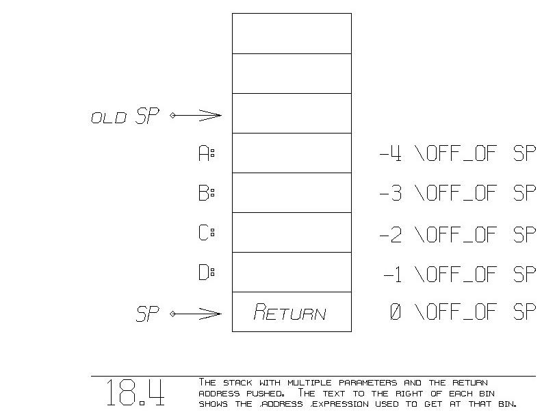 We pass multiple parameters by pushing each one onto the stack. The
last parameter pushed is accessed within the function via the address
expression "-1 \OFF_OF SP", like before. The second to last parameter
resides at "-2 \OFF_OF SP". In general, the K'th to the last parameter
resides at "-K \OFF_OF SP". See figure 18.4.
As before, the called function associates each of these address
expressions with the name of the parameter. For example, the following
function definition makes the association of address expressions to
its parameters:
DEFINE F( A,B,C: INT D: REAL ):
"D now denotes -1 \OFF_OF SP"
"C now denotes -2 \OFF_OF SP"
"B now denotes -3 \OFF_OF SP"
"A now denotes -4 \OFF_OF SP"
...
ENDDEFN
Upon leaving, this function restores RETURN and then pops the four
parameters off the stack:
LOAD( RETURN , 0 \OFF_OF SP );
SUB( SP , ADDRESS_OF( 5 ) );
Figure 18.4 shows the stack after entry and having pushed RETURN onto
the stack. To restore the old SP, we decrement SP by 5. We always
decrement SP by 1 plus the number of parameters, so as to effectively
pop all the parameters and the one return address off the stack.
18.2.5
The Frame Pointer (FP)
Our function calling method is nearly correct. Consider the
following function call to G within the body of F:
DEFINE F( A,B,C: INT D: REAL ):
"D now denotes -1 \OFF_OF SP"
"C now denotes -2 \OFF_OF SP"
"B now denotes -3 \OFF_OF SP"
"A now denotes -4 \OFF_OF SP"
G(A,B);
ENDDEFN
We pass multiple parameters by pushing each one onto the stack. The
last parameter pushed is accessed within the function via the address
expression "-1 \OFF_OF SP", like before. The second to last parameter
resides at "-2 \OFF_OF SP". In general, the K'th to the last parameter
resides at "-K \OFF_OF SP". See figure 18.4.
As before, the called function associates each of these address
expressions with the name of the parameter. For example, the following
function definition makes the association of address expressions to
its parameters:
DEFINE F( A,B,C: INT D: REAL ):
"D now denotes -1 \OFF_OF SP"
"C now denotes -2 \OFF_OF SP"
"B now denotes -3 \OFF_OF SP"
"A now denotes -4 \OFF_OF SP"
...
ENDDEFN
Upon leaving, this function restores RETURN and then pops the four
parameters off the stack:
LOAD( RETURN , 0 \OFF_OF SP );
SUB( SP , ADDRESS_OF( 5 ) );
Figure 18.4 shows the stack after entry and having pushed RETURN onto
the stack. To restore the old SP, we decrement SP by 5. We always
decrement SP by 1 plus the number of parameters, so as to effectively
pop all the parameters and the one return address off the stack.
18.2.5
The Frame Pointer (FP)
Our function calling method is nearly correct. Consider the
following function call to G within the body of F:
DEFINE F( A,B,C: INT D: REAL ):
"D now denotes -1 \OFF_OF SP"
"C now denotes -2 \OFF_OF SP"
"B now denotes -3 \OFF_OF SP"
"A now denotes -4 \OFF_OF SP"
G(A,B);
ENDDEFN
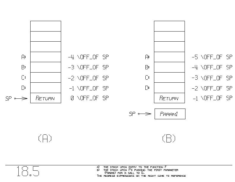 As we are about to call G, the stack looks like figure 18.5(a). Let's
call G. We first push the first parameter, A, onto the stack. Figure
18.5(b) shows the status. Notice how "-1 \OFF_OF SP" has moved up one
bin. This is natural since we've incremented SP. Unfortunately,
having pushed A already onto the stack, SP has moved, and so the
address expression "-3 \OFF_OF SP" no longer denotes B, but C instead
(figure 18.5(b))!
When we are in the middle of pushing parameters onto the stack, SP
moves, which throws off our address expression assignments.
One way to solve this problem is to introduce another register
different from SP which "freezes" the value in SP. We call that
register FP, short for "frozen pointer" or "frame pointer".
Let's have the beginning of all our functions set FP to SP first thing:
F: ADD( SP, ADDRESS_OF(1) ); "Push RETURN as before"
STORE( RETURN, 0 \OFF_OF SP );
LOAD( FP, SP ); "New: set FP to SP"
"the function body:"
...
Now throughout this functions body, let's use FP instead of SP. We
associate with the K'th parameter the address expression:
K-5 \OFF_OF FP instead of K-5 \OFF_OF SP
As we are about to call G, the stack looks like figure 18.5(a). Let's
call G. We first push the first parameter, A, onto the stack. Figure
18.5(b) shows the status. Notice how "-1 \OFF_OF SP" has moved up one
bin. This is natural since we've incremented SP. Unfortunately,
having pushed A already onto the stack, SP has moved, and so the
address expression "-3 \OFF_OF SP" no longer denotes B, but C instead
(figure 18.5(b))!
When we are in the middle of pushing parameters onto the stack, SP
moves, which throws off our address expression assignments.
One way to solve this problem is to introduce another register
different from SP which "freezes" the value in SP. We call that
register FP, short for "frozen pointer" or "frame pointer".
Let's have the beginning of all our functions set FP to SP first thing:
F: ADD( SP, ADDRESS_OF(1) ); "Push RETURN as before"
STORE( RETURN, 0 \OFF_OF SP );
LOAD( FP, SP ); "New: set FP to SP"
"the function body:"
...
Now throughout this functions body, let's use FP instead of SP. We
associate with the K'th parameter the address expression:
K-5 \OFF_OF FP instead of K-5 \OFF_OF SP
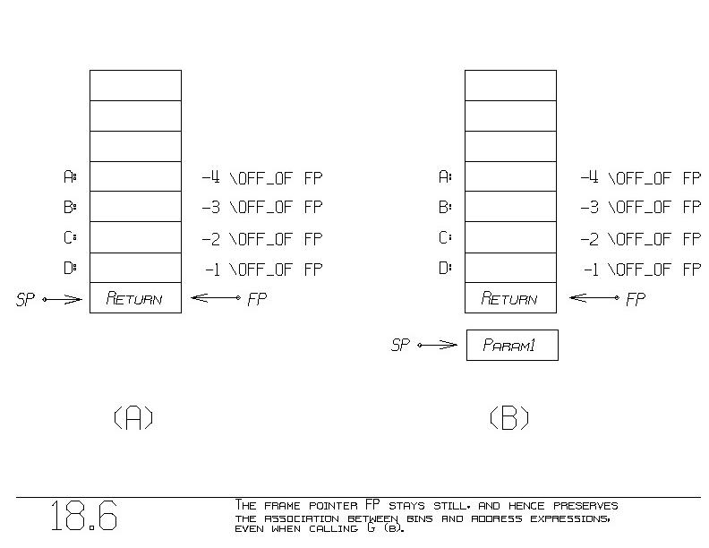 The first parameter (K=1) resides at "-4 \OFF_OF FP". Figure 18.6
is an updated 18.5. Part (a) shows the stack after F is called and its
initial program fragment is done executing. The only thing new is the
introduction of FP. Part (b) shows us in the middle of calling G. SP
has been incremented, but that no longer hurts us. Upon pushing the
second parameter, B, the address expression "-3 \OFF_OF FP" for B still
denotes F's input parameter B.
18.2.5.1
Saving FP
Since we will be using FP to reference our parameters, we expect FP
to remain unchanged throughout our function body. That is, even after
we call G and G returns, we expect FP to be what it was.
Unfortunately, as we've set things up so far, FP will be changed by
the first function we call. (Recall, that function's initial program
fragment overwrites FP with a new value from SP. Upon return from
that function call, FP is no longer what we expect it to be).
We must therefore have each function save and later restore the value
in FP, so that calls leave FP unchanged.
The first parameter (K=1) resides at "-4 \OFF_OF FP". Figure 18.6
is an updated 18.5. Part (a) shows the stack after F is called and its
initial program fragment is done executing. The only thing new is the
introduction of FP. Part (b) shows us in the middle of calling G. SP
has been incremented, but that no longer hurts us. Upon pushing the
second parameter, B, the address expression "-3 \OFF_OF FP" for B still
denotes F's input parameter B.
18.2.5.1
Saving FP
Since we will be using FP to reference our parameters, we expect FP
to remain unchanged throughout our function body. That is, even after
we call G and G returns, we expect FP to be what it was.
Unfortunately, as we've set things up so far, FP will be changed by
the first function we call. (Recall, that function's initial program
fragment overwrites FP with a new value from SP. Upon return from
that function call, FP is no longer what we expect it to be).
We must therefore have each function save and later restore the value
in FP, so that calls leave FP unchanged.
 We now save on the stack not only RETURN, but FP as well. Figure
18.7(a) shows our desired situation after entry into our function,
having executed our initial program fragment. The following is our new
function entry and exit:
F: ADD( SP , ADDRESS_OF(1) ); "Push RETURN"
STORE( RETURN , 0 \OFF_OF SP );
ADD( SP , ADDRESS_OF(1) ); "Push FP"
STORE( FP, 0 \OFF_OF SP );
LOAD( FP, SP ); "Set our FP"
"function body:"
...
"Return process:"
LOAD( RETURN, -1 \OFF_OF FP ); "Restore RETURN"
LOAD( FP, 0 \OFF_OF FP ); "Restore FP"
SUB( SP , ADDRESS_OF( 2 + number_of_arguments ) );
"Restore SP to status before
our being called"
JUMP( 0 \OFF_OF RETURN );
Notice that we decrement SP by two plus the number of arguments in this
function. The two takes off the storage used for RETURN and old FP.
The rest removes the parameters from the stack.
As figure 18.7(a) shows, we must now assign slightly different address
expressions to our parameters:
Parameter K is now K-6 \OFF_OF FP
We now have a correct function calling mechanism.
BOX: What kind of address expression is associated with
BOX: parameter variables?
BOX:
BOX: Why is FP necessary (assuming that pushes and pops can
BOX: occur)?
BOX:
BOX: Upon function exit, how far is SP decremented?
18.2.6
Implementing Local Variables
Now we are ready to introduce local variables. Consider the function:
DEFINE F( A,B,C: INT D: REAL ):
BEGIN VAR X,Y,Z = REAL;
"body"
END
ENDDEFN
Figure 18.7(a) shows how F's initial program fragment leaves the stack.
This accounts for parameters.
We now save on the stack not only RETURN, but FP as well. Figure
18.7(a) shows our desired situation after entry into our function,
having executed our initial program fragment. The following is our new
function entry and exit:
F: ADD( SP , ADDRESS_OF(1) ); "Push RETURN"
STORE( RETURN , 0 \OFF_OF SP );
ADD( SP , ADDRESS_OF(1) ); "Push FP"
STORE( FP, 0 \OFF_OF SP );
LOAD( FP, SP ); "Set our FP"
"function body:"
...
"Return process:"
LOAD( RETURN, -1 \OFF_OF FP ); "Restore RETURN"
LOAD( FP, 0 \OFF_OF FP ); "Restore FP"
SUB( SP , ADDRESS_OF( 2 + number_of_arguments ) );
"Restore SP to status before
our being called"
JUMP( 0 \OFF_OF RETURN );
Notice that we decrement SP by two plus the number of arguments in this
function. The two takes off the storage used for RETURN and old FP.
The rest removes the parameters from the stack.
As figure 18.7(a) shows, we must now assign slightly different address
expressions to our parameters:
Parameter K is now K-6 \OFF_OF FP
We now have a correct function calling mechanism.
BOX: What kind of address expression is associated with
BOX: parameter variables?
BOX:
BOX: Why is FP necessary (assuming that pushes and pops can
BOX: occur)?
BOX:
BOX: Upon function exit, how far is SP decremented?
18.2.6
Implementing Local Variables
Now we are ready to introduce local variables. Consider the function:
DEFINE F( A,B,C: INT D: REAL ):
BEGIN VAR X,Y,Z = REAL;
"body"
END
ENDDEFN
Figure 18.7(a) shows how F's initial program fragment leaves the stack.
This accounts for parameters.
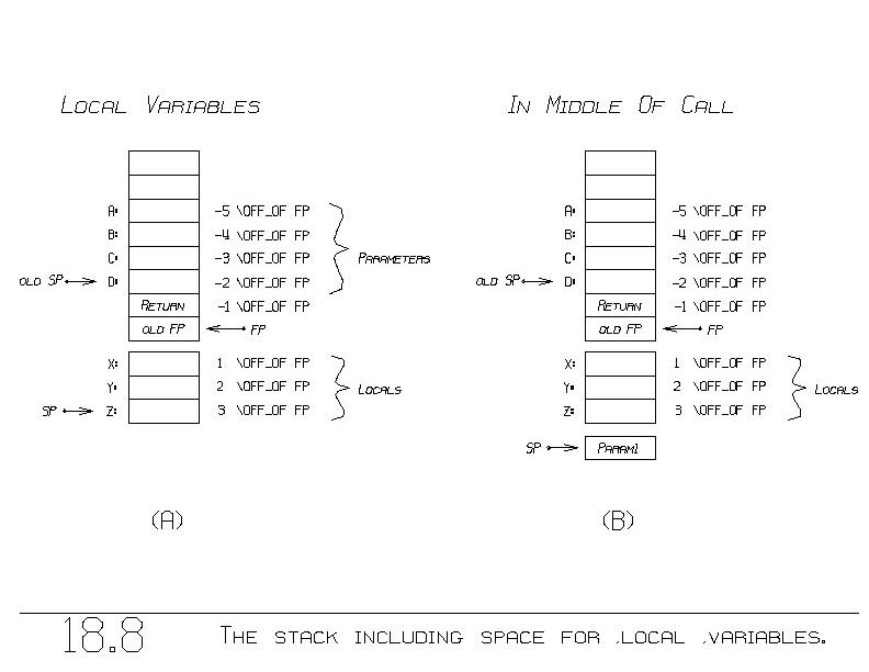 Figure 18.8(a) shows how we would like it to be, so as to provide
storage for our three local variables X, Y, and Z. We modify once
more F's initial and final program fragments:
F: "unchanged..."
ADD( SP , ADDRESS_OF(1) ); "Push RETURN"
STORE( RETURN, 0 \OFF_OF SP );
ADD( SP , ADDRESS_OF(1) ); "Push FP"
STORE( FP, 0 \OFF_OF SP );
LOAD( FP, SP ); " Set FP for us "
"new..."
ADD( SP, ADDRESS_OF( number_of_locals ) );
" Allocate space for locals"
"function body:"
...
"Return process:"
LOAD( RETURN , -1 \OFF_OF FP ); " Restore RETURN "
LOAD( FP , 0 \OFF_OF FP ); " Restore FP "
SUB( SP, ADDRESS_OF( 2 + number_of_locals
+ number_of_arguments ) );
JUMP( 0 \OFF_OF RETURN );
The initial program fragment has a new ADD, which increments SP by
the number of locals, thus achieving figure 18.8(a). The final program
fragment is changed so as to decrement SP enough to deallocate the
locals, the parameters, and the two bins that hold RETURN and old FP.
18.2.6.1
A More Efficient Rendition
For purposes of efficiency, let's rewrite the initial program fragment
nearly equivalently as follows:
F: STORE( RETURN , 1 \OFF_OF SP ); "Save RETURN"
STORE( FP , 2 \OFF_OF SP ); "Save FP"
LOAD( FP, SP ); "Set FP for us"
ADD( SP , ADDRESS_OF( 2 + number_of_locals ); "Set SP"
"body:"
...
Figure 18.8(a) shows how we would like it to be, so as to provide
storage for our three local variables X, Y, and Z. We modify once
more F's initial and final program fragments:
F: "unchanged..."
ADD( SP , ADDRESS_OF(1) ); "Push RETURN"
STORE( RETURN, 0 \OFF_OF SP );
ADD( SP , ADDRESS_OF(1) ); "Push FP"
STORE( FP, 0 \OFF_OF SP );
LOAD( FP, SP ); " Set FP for us "
"new..."
ADD( SP, ADDRESS_OF( number_of_locals ) );
" Allocate space for locals"
"function body:"
...
"Return process:"
LOAD( RETURN , -1 \OFF_OF FP ); " Restore RETURN "
LOAD( FP , 0 \OFF_OF FP ); " Restore FP "
SUB( SP, ADDRESS_OF( 2 + number_of_locals
+ number_of_arguments ) );
JUMP( 0 \OFF_OF RETURN );
The initial program fragment has a new ADD, which increments SP by
the number of locals, thus achieving figure 18.8(a). The final program
fragment is changed so as to decrement SP enough to deallocate the
locals, the parameters, and the two bins that hold RETURN and old FP.
18.2.6.1
A More Efficient Rendition
For purposes of efficiency, let's rewrite the initial program fragment
nearly equivalently as follows:
F: STORE( RETURN , 1 \OFF_OF SP ); "Save RETURN"
STORE( FP , 2 \OFF_OF SP ); "Save FP"
LOAD( FP, SP ); "Set FP for us"
ADD( SP , ADDRESS_OF( 2 + number_of_locals ); "Set SP"
"body:"
...
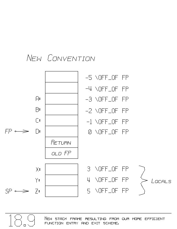 This more efficient program fragment removes the first two ADD
instructions, and leaves things as shown in figure 18.9.
As indicated in the figure:
the K'th parameter can be accessed by K-4 \OFF_OF FP
and
the I'th local can be accessed by I+2 \OFF_OF FP
The updated final program fragment is:
"Return process:"
LOAD( RETURN , 1 \OFF_OF FP ); " Restore RETURN "
LOAD( FP , 2 \OFF_OF FP ); " Restore FP "
SUB( SP, ADDRESS_OF( 2 + number_of_locals
+ number_of_arguments ) );
JUMP( 0 \OFF_OF RETURN );
We now have a function calling mechanism which accounts for locals and
parameters.
BOX: What kind of address expression is associated with
BOX: local variables?
BOX:
BOX: Why is it that a function can call itself recursively,
BOX: and still have local variables that don't interfere
BOX: with one another thru the recursive call?
BOX:
BOX: What two values, besides parameters and locals, are
BOX: saved on the stack?
BOX:
BOX: Does this calling convention have to be implemented in
BOX: software (as we have done) or can it be done in
BOX: hardware? What would be the advantages and
BOX: disadvantages?
18.2.7
Other Conventions For Parameters And Locals
Section 19.9 introduces another way to implement parameters and locals.
This more efficient program fragment removes the first two ADD
instructions, and leaves things as shown in figure 18.9.
As indicated in the figure:
the K'th parameter can be accessed by K-4 \OFF_OF FP
and
the I'th local can be accessed by I+2 \OFF_OF FP
The updated final program fragment is:
"Return process:"
LOAD( RETURN , 1 \OFF_OF FP ); " Restore RETURN "
LOAD( FP , 2 \OFF_OF FP ); " Restore FP "
SUB( SP, ADDRESS_OF( 2 + number_of_locals
+ number_of_arguments ) );
JUMP( 0 \OFF_OF RETURN );
We now have a function calling mechanism which accounts for locals and
parameters.
BOX: What kind of address expression is associated with
BOX: local variables?
BOX:
BOX: Why is it that a function can call itself recursively,
BOX: and still have local variables that don't interfere
BOX: with one another thru the recursive call?
BOX:
BOX: What two values, besides parameters and locals, are
BOX: saved on the stack?
BOX:
BOX: Does this calling convention have to be implemented in
BOX: software (as we have done) or can it be done in
BOX: hardware? What would be the advantages and
BOX: disadvantages?
18.2.7
Other Conventions For Parameters And Locals
Section 19.9 introduces another way to implement parameters and locals.